A Dozen Excel Time-Savers
Q. What are some of your favorite tricks for getting the most out of Excel?
A. Excel has been a staple of this column since its launch almost 20 years ago, and I've provided innumerable Excel tips myself since taking it over from Stanley Zarowin in January 2011. I recommend you search the JofA website (or browse journalofaccountancy.com/excel), as almost all of those Excel tips and tricks are still valid today, though the menu options for accessing those tricks may have changed.
To answer your question, I've compiled a list of a dozen Excel tricks that will help any CPA become more efficient and effective. (If you are an avid Excel user, you are probably already familiar with most of these meat-and-potatoes workbook tips, but they are worth reviewing in any case.) You can also view my video demonstrating all 12 of these techniques.
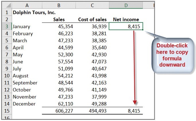
- Double-click to fill down: A trick I frequently use is double-clicking the Fill Handle to copy downward. The Fill Handle is the small green square located in the bottom right corner of your selection — be it one cell or a larger group of cells. Double-clicking the Fill Handle causes the selected text, formula, or data to be copied downward, with different behaviors resulting depending on the contents of the cell. For example, if the data happen to be a formula (as pictured below), the formula will copy downward to fill all empty cells when there are data contained in the adjacent column's cells (or when there are data in more distant columns, as long as they are connected by column headings).
If the data to be copied down are ordinary text, then the text will be repeated. If the data to be copied down are text included in a Custom List, such as the words "January," "Monday," or "Quarter 1," then the data copied down will be the next value in that list. For example, double-clicking the Fill Handle of a cell containing the word January will produce the words February, March, April, and so on downward, as long as there are data in adjacent (or connected) columns.
If the data range to be copied contains two values, then Excel will extrapolate the value trend. For example, the values 1 and 2 will be copied downward as 3, 4, 5, and so on. If the data range to be copied contains three values or more, then Excel will use linear regression to calculate the new values, which can be useful for projecting forecasts based on historical values.
2. Paste as unformatted text: By default, Excel pastes text and data you've copied with their original formatting, which is not always what you want. You can avoid reformatting by pasting your text or data as Unformatted Text (as pictured below). The pasted text or data will adopt the default formatting of the target area where they are being pasted.
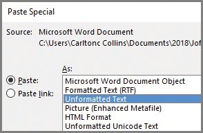
For example, let's say you want to copy and paste blue text with a 6.5-point Helvetica font to an area in Excel with the default formatting of a black, 12-point Calibri font. If you use the Paste as Unformatted Text option, the pasted data will automatically display as black, 12-point Calibri font — thereby saving you the extra effort required to reformat the pasted text or data.
3. Double-click to increase column width: A good time-saver is to double-click the right edge of a column in its header label area, as pictured below, to automatically adjust the column's width to the largest contents contained in the column.
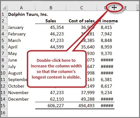
Further, you can select multiple columns and then double-click just one of the selected columns as described above to adjust all selected columns simultaneously. In this case, the selected columns may then possibly appear as different widths, depending upon the length of the data in those columns.
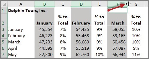
- Make all column widths even: Another column width trick is to select multiple columns and then manually adjust the width of one column to simultaneously adjust the width of all selected columns. In this case, the selected columns will all be adjusted to the same width, regardless of the length of the data in those columns. This trick works even when your columns aren't contiguous. For example, as pictured below, I've selected the data columns B, D, and F (by holding down the Ctrl key as I selected each column), and I then adjusted the width of one column (as shown by the red arrow), which automatically adjusted the width of all selected columns, making them the same size.
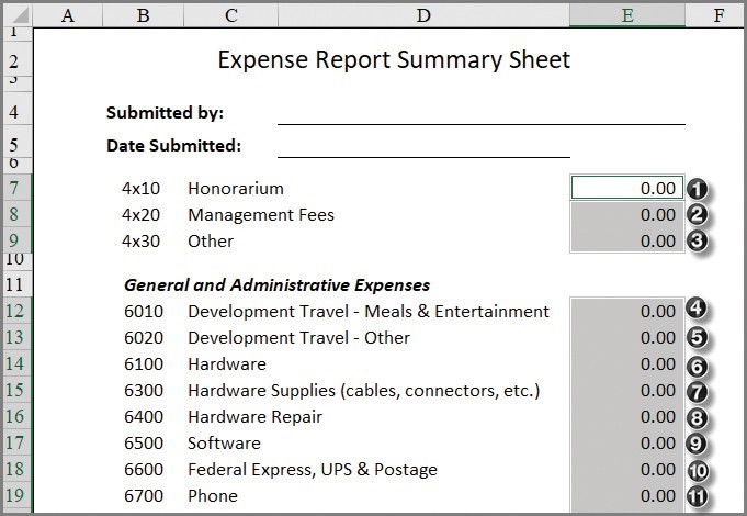
- Selecting cells where you want to enter data: For a worksheet where you want to enter data into multiple cells (either adjacent or scattered across your worksheet), you might find it useful to first select all of those blank cells while holding down the Ctrl key; thereafter, you can enter data into each selected cell and advance to the next cell by pressing the Enter key. This trick then enables you to use your computer's number pad like a 10-key calculator, where your cursor automatically navigates to the next input cell upon pressing the Enter key. For example, in the worksheet below I've selected cells E7 through E9 and cells E12 through E19 (numbered 1 through 11 below), and my cursor is positioned at cell E7. From this range selection, I can input data into E7 and press the Enter key to both enter the data and move the cursor automatically to the next selected cell — E8 in this example. Again, I can enter a value into cell E8 and then press the Enter key to jump to cell E9 and so on to cells E12, E13, etc. This approach eliminates the need to navigate to each new cell.
6. Custom lists: Excel enables you to create a Custom List of those names, labels, or lists you frequently use — such as departments, accounts, employees, locations, etc. Thereafter, you can re-create those lists in any workbook (old or new) simply by entering one of the names from your Custom List and dragging the Fill Handle to complete the list.
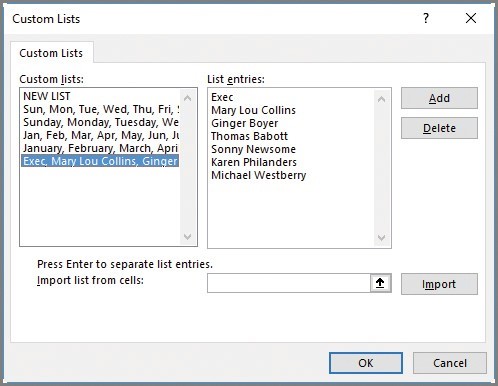
To create a Custom List, from the File tab select Options, Advanced, and scroll down to the General section and select the Edit Custom Lists button to display the Custom Lists dialog box pictured at the bottom of the previous page. Next, in the List entries section, type the list you frequently use, such as the names of your executive team, an example of which is demonstrated below. (Notice in this example that I've begun my custom list with the word Exec, which is my shortcut for my company's Executive Team.) Be sure to click the Add and OK buttons to complete the custom list creationprocess.
I can then type the word Exec into any workbook and drag the Fill Handle in any direction to produce this list, as suggested in the screenshot below.
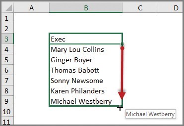
7. Use Scroll Tips to figure out where to stop: Note in the screenshot above that Scroll Tips are pop-up indicators that display the value that AutoFill will insert in each cell. This makes it easier to paint a fill range of appropriate size.
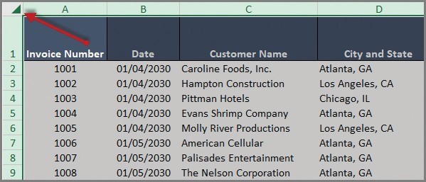
8. Select an entire worksheet: The fastest way to select an entire worksheet (for copying or deleting that worksheet, for example) is to click the upper left corner of the worksheet — between the header and row label areas as indicated by the red arrow below.
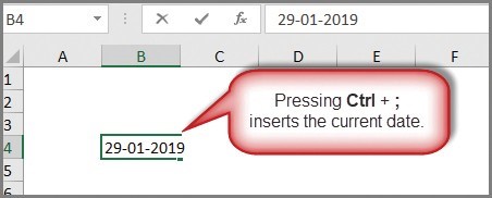
9. Insert the current date: Quickly insert today's date by pressing the Ctrl+; (semicolon) key combination, as pictured at the top of the next column.
10. Insert a comment: Quickly insert a comment by pressing the Shift+F2 key combination.
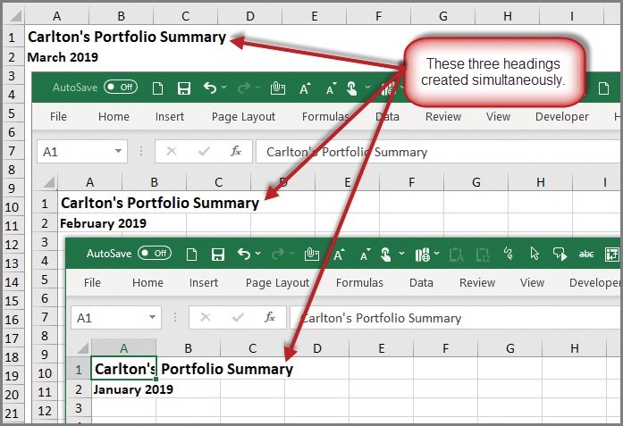
11. Type across multiple worksheets simultaneously: You can enter text or data across multiple worksheets at the same time by first holding down the Ctrl key, selecting the tabs of the worksheets where you want to type, and then entering the desired text or data. For example, if you have 12 worksheets that you want to contain the same company name and date, you could select every worksheet and then enter the report title in the upper left corner on one sheet, and that entry is automatically duplicated on the other 11 worksheets, as suggested in the screenshot below.
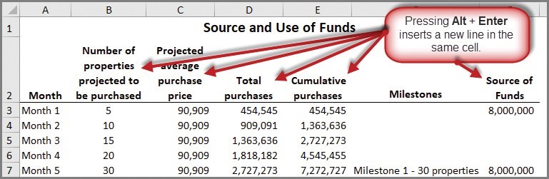
12. Enter multiple lines in a cell: When typing into a cell, insert a line break by pressing the Alt+Enter key combination, which effectively inserts a new row in that cell. This trick comes in handy when entering longer titles as column headings, an example of which is pictured below. (This same effect can also be achieved by formatting the cell to Wrap text.)
(Source: AICPA - CPA Letter Daily - Journal of Accountancy - May 13, 2019)